

Geospatial data analysis is critical across all sectors of investigations, from Law Enforcement to National Security, Cybersecurity and more.
Siren provides multiple components that have mapping capabilities, namely the Enhanced Coordinate Map (a visualization that can be added to any dashboard) and the Map Mode of the Graph Browser.
This post will introduce the Siren Enhanced Coordinate Map (ECM). We will explore some of the key features of this visualisation including the loading of GeoJSON, configuration of the default Base Layer. We will also provide insight for configuring and working with layers in ECM and how dashboards can be filtered by creating geo filters from ECM.
There are various sources for data on ECM. At the core, it displays data from indices (stored in the backend Elasticsearch) linked to Entity Tables. Additionally, you can ingest overlay and point data that contain spatial information (Stored Layers), from tile servers (WMS/WMTS) or from Map Services (WFS).
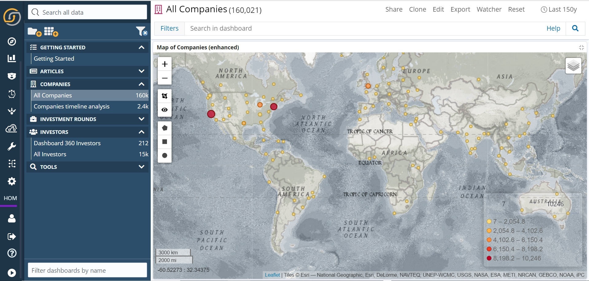
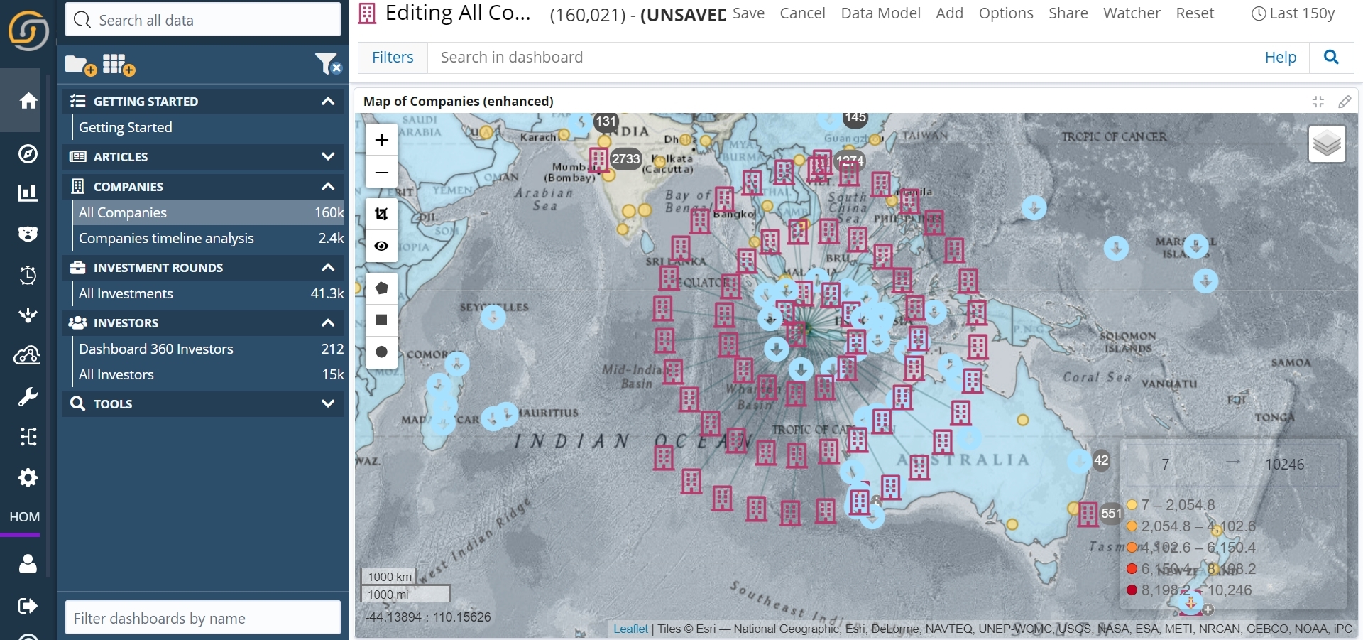
The ECM visualisation can then be added to dashboards, where they become fully interactive visualisations, allowing users to geographically view and filter data, or even add new data by simply dragging other dashboards onto the map.
The ECM by default displays an Aggregation layer and a Geo Filter layer. The Aggregation layer is based on the configured main search for the ECM visualisation and is created by aggregating geographical data in real time by high performance backend functions like Elasticsearch geohash aggregation bucket. The Geo Filters overlay is a visual representation of geographical filters which have been created directly by users on that ECM.
Geo filters added to the dashboard are applied to all other present visualisations. They also apply when passed to another dashboard via the Relational Navigator visualisation. An option can be configured to toggle whether dashboard filters are applied to Point Of Interest Layers. Geo filters do not apply to layers from WFS or Stored Layer sources. However, these layers are useful as a way to provide context about other relevant information during the investigation. Examples of all of the above will be provided, so keep reading!
Additional tile server layers can also be configured to allow for quick toggling between the default Base Layer and others. For example, roads, satellite views, or a hybrid from sources such as Google Maps, Bing Maps, or OpenStreetMap.
Configuring the Map with Tile Server in Siren:
Let’s start by configuring the default Base Layer. The default Base Layer will be visible even if your map contains no other configuration. We will use the ESRI World Street Map as an example. Of course, you can configure Siren Investigate to use your own tile service depending on your requirement. You can also use existing free or paid tilemap providers, or build your own Tile Server.
Note – if your tile server supports WMS/WMTS, it is compatible with Siren Investigate.
The tilemap settings for configuring ESRI World Street Map as the default Base Layer are provided below. This can be pasted directly into the investigate.yml file:
tilemap:
  url: 'https://server.arcgisonline.com/ArcGIS/rest/services/NatGeo_World_Map/MapServer/tile/{z}/{y}/{x}'
  options:
    attribution: 'Tiles © Esri — National Geographic, Esri, DeLorme, NAVTEQ, UNEP-WCMC, USGS, NASA, ESA, METI, NRCAN, GEBCO, NOAA, iPC'
    subdomains: ['a']
    minZoom: 0
    maxZoom: 16
Aggregation Layer Tooltips:
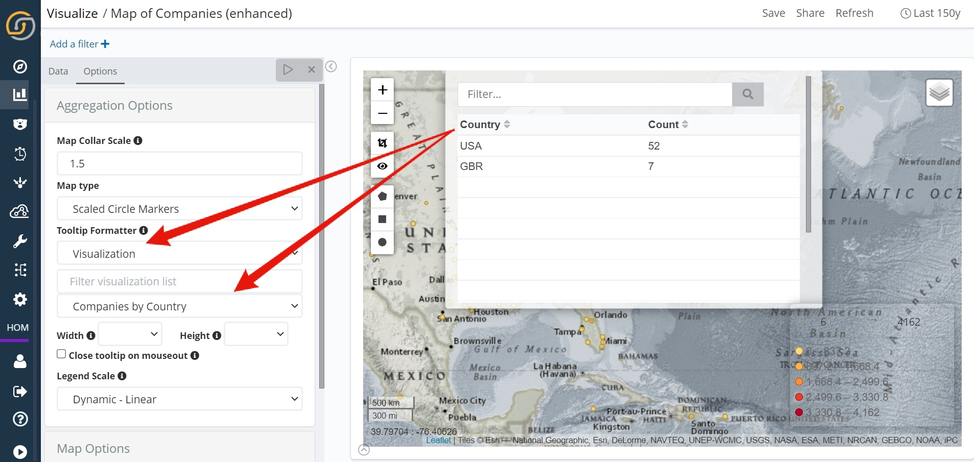
Metric and visualisation tooltip types are configurable. Metrics provide summary statistics based on the count of documents or any of the average, sum, min, max or unique count based on a specified numerical field. Most visualisations that are configured to the same index as the ECM can be added as ECM tooltips. The data within these visualisations correspond to just the data within the Aggregation marker (i.e. the geohash aggregation bucket) hovered on.
Stored Layers:
There are two provided methods for loading GeoJSON files into Elasticsearch as Stored Layers. These are Folder Structure and the Spatial Path. Both will accept files of type JSON or GeoJSON. The methods differ in how their spatial_path is determined, but once they have been ingested into Elasticsearch, they function in the same way. The most suitable approach depends on the form of your current data.
Note – Custom scripts can be produced for ingesting data as Stored Layers in Investigate. As long as an index contains a geo field type (geo_point for points or geo_shape for lines or polygons) and is prefixed with .map__, it will be treated as a Stored Layer
We will be using the Folder Structure because our GeoJSON data does not have a spatial_path attribute within the properties object of each GeoJSON feature.
Load GeoJSON into Elasticsearch:
- The GeoJSON files we will use in this example can be downloaded here. We are using:
- populated places simple – Sample dataset of some of the world’s largest cities
- admin 0 countries – Sample dataset of some of the world’s largest countries
- Create the folder structure below and place the downloaded GeoJSONs into it.
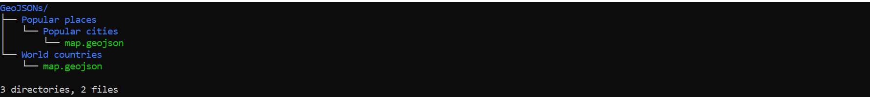
- The script to ingest GeoJSONs can be executed from the Siren Investigate folder. There are configurable arguments and the command below will log them to the console:
bin/load_map_reference_indices.sh --help- For our example, run the command below to load GeoJSON into the Elasticsearch:
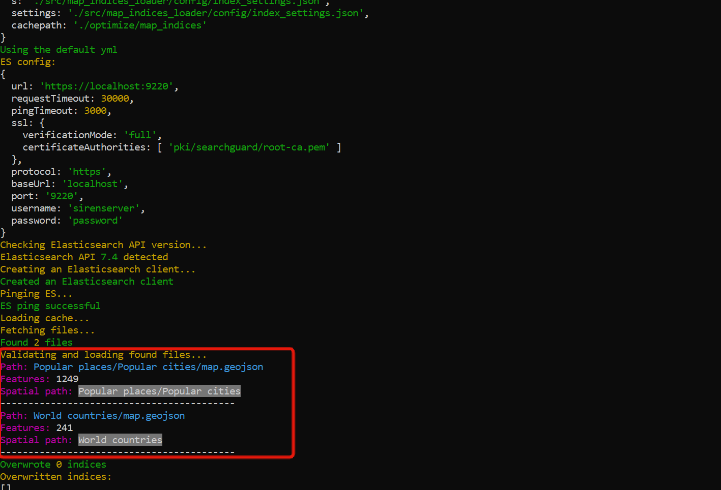
/bin/load_map_reference_indices.sh -p "<path to your GeoJSON folder>/geojson/" --debug --structure --overwrite The -p argument is the path to the GeoJSON folder and is required. Other argument details are described in the documentation here. The console output below is a successful load (with –debug argument).
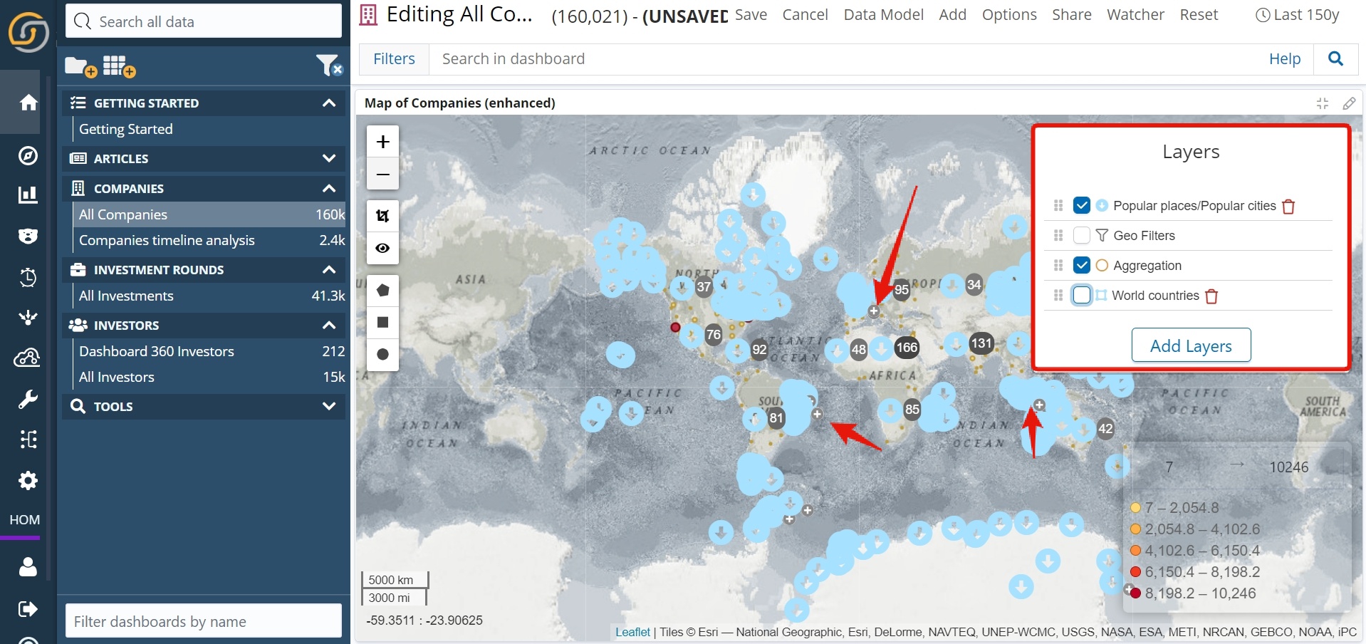
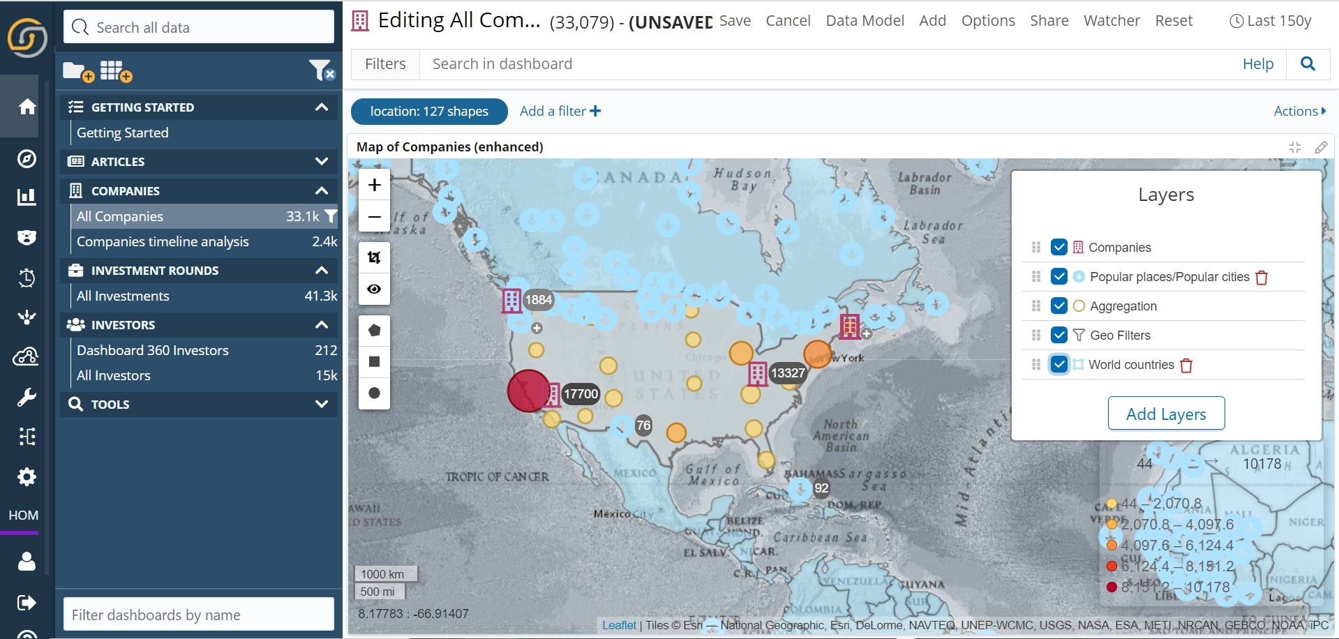
Visualise the Stored Layers in ECM:
The Layer Control is located in the top-right corner of any ECM. When clicked on, it allows you to select which Stored Layers (i.e. from the example above, the GeoJSONs that we imported) can be added to the map. Select the ‘Populated cities’ and ‘World Countries’ Stored layer and click ‘Add and Display’. This will add it to the map and make it visible. If you are loading many layers, the ‘Add’ option might be useful, as rendering layers on the map can take time.
Point of Interest Layers:
Point of Interest (POI) layers are useful for representing other searches (that contain a geo_point or geo_shape type) on the map. In the example below, we are using the companies index to represent a Point of Interest layer. The ‘apply filters’ option is checked which means that filters from our dashboard will also filter this POI layer.
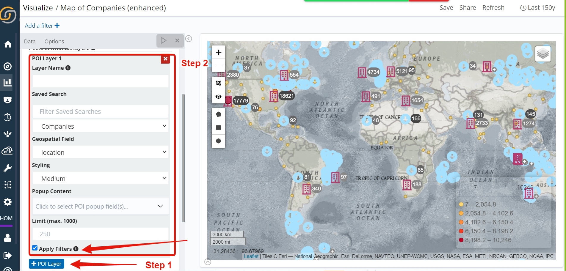
It is also possible to create POIs by dragging a dashboard which has a main search containing a geo_point field.
Marker clustering:
Marker clustering is used for point layers coming from either POI or Stored Layer sources. It allows all points on that particular layer to be represented at once.
The image below shows the Populated places Stored Layer on the Map. As the layer contains many points that would overlap at the current zoom level, it is showing the areas where there are higher densities of points as Marker clusters with a number on the cluster representing the amount of points:
In the areas where there are lower point densities, but still contain overlapping points, grouping happens. You know they are grouped because there is a + to the right of the marker. These can be ‘exploded’ by clicking on them, which is also known as Spiderfying.
Layer Ordering:
Layers are drawn on the map in the same order they are in the Layer Control (points always show in front of other layers). Layers can be ordered by clicking the drag handle to the left of any checkbox and dragging them to the desired position.
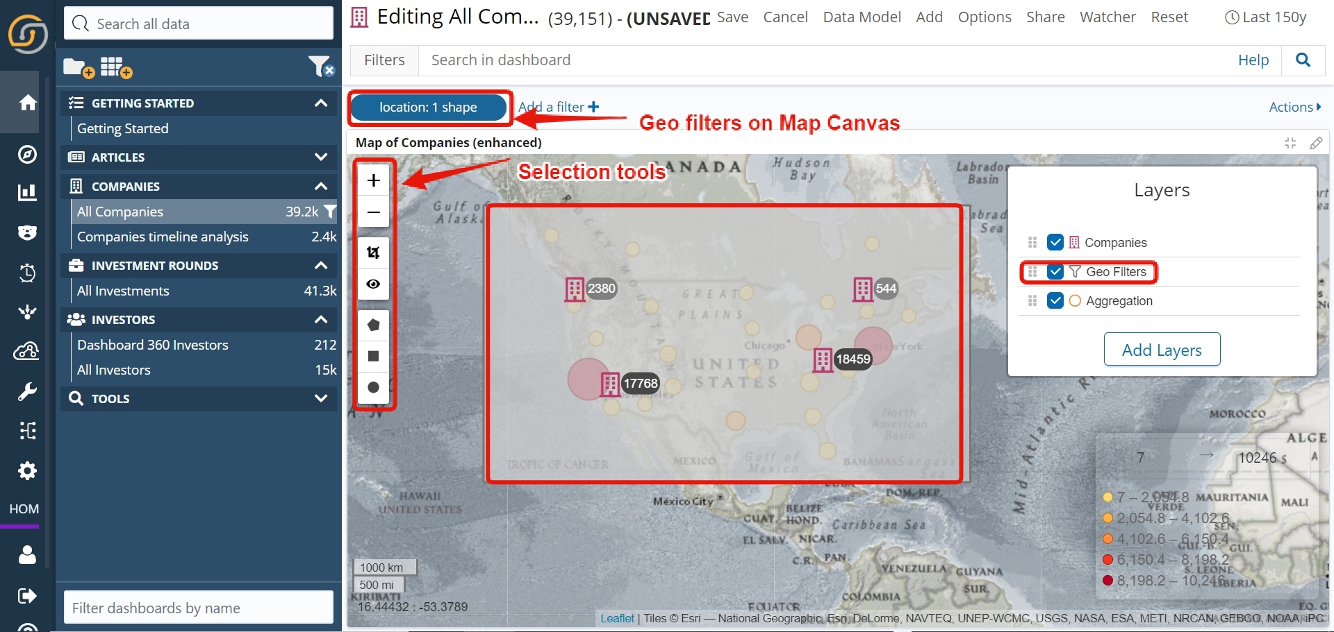
Geo filters:
Geo filters can be used to spatially filter the Aggregation layer or POI layers (that have the ‘apply filters’ option checked). When on dashboards, other visualisations are also filtered by geo filters.
They can be created by either using the selection tools or by clicking polygons rendered on the map.
Selection tools:
An example of the selection tools approach is shown below where the Aggregation and POI layers are filtered by drawing a rectangle.
Clicking polygon geo filters:
When polygons are added to the map (either from POI, Stored Layer or WFS sources), clicking on them will create a geo filter.
Multiple geo filters:
It is possible to add multiple geo filters to the same Map. When a second geo filter is added, a modal will appear where you can select how you want the second filter to be added.
- Overwrite existing filter – Can be useful if you’ve accidentally created or would like to quickly replace the one currently active filter
- Create new filter – Can be useful for quickly toggling between multiple filters (by clicking the checkboxes to toggle on and off)
- Combine with existing filters – If you would like to always use the new filter with the one currently active filter, you can combine them
Even if there are multiple geo filters already on your dashboard. It is possible to overwrite or combine with a specific geo filter by having just that one enabled. Then by creating a new geo filter, the modal will appear and the option selected will apply to the one enabled geo filter.
Below, the Aggregation layer and companies POI gets filtered with the applied Geo-filter, while all Populated places remain. This is because Populated places is a Stored Layer and its purpose is to provide context for the Aggregation and POI layers.
Conclusion:
Geospatial analysis is critical for many kinds of investigation. If you want to explore the Siren dashboard with the map yourself, feel free to download the Siren Platform Demo Data and explore the Enhanced Coordinate Map in Siren.
Resources:
Enhanced Tilemap Configuration
Written by: Manu Agarwal and Edwin Corrigan


